



Live demos of what IKPy can do (click on the image below to see the video):

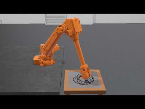
Also, a presentation of IKPy: Presentation.
With IKPy, you can:
- Compute the Inverse Kinematics of every existing robot.
- Compute the Inverse Kinematics in position, orientation, or both
- Define your kinematic chain using arbitrary representations: DH (Denavit–Hartenberg), URDF, custom...
- Automatically import a kinematic chain from a URDF file or a MuJoCo MJCF file.
- Support for arbitrary joint types:
revolute,prismaticand more to come in the future - Use pre-configured robots, such as baxter or the poppy-torso
- IKPy is precise (up to 7 digits): the only limitation being your underlying model's precision, and fast: from 7 ms to 50 ms (depending on your precision) for a complete IK computation.
- Plot your kinematic chain: no need to use a real robot (or a simulator) to test your algorithms!
- Define your own Inverse Kinematics methods.
- Utils to parse and analyze URDF files:

Moreover, IKPy is a pure-Python library: the install is a matter of seconds, and no compiling is required.
IKPy now includes an optional JAX backend for accelerated inverse kinematics using automatic differentiation.
| Scenario | Speedup vs NumPy |
|---|---|
| Single target (complex chains) | 1.5-4x faster |
| Trajectory tracking (warm start) | 2-3x faster |
| Cold start | More robust (fewer local minima) |
The JAX backend uses an analytical Jacobian computed via autodiff, which provides:
- Faster convergence on difficult targets
- Better robustness against local minima
- Significant speedup on robots with 5+ joints
pip install 'ikpy[jax]'from ikpy.chain import Chain
# Load your robot
chain = Chain.from_urdf_file("my_robot.urdf")
# Use JAX backend for IK
result = chain.inverse_kinematics(
target_position=[0.5, 0.2, 0.3],
backend="jax" # Use JAX instead of NumPy
)
# Trajectory tracking with warm start (recommended)
current_joints = None
for target in trajectory:
result = chain.inverse_kinematics(
target_position=target,
initial_position=current_joints,
backend="jax"
)
current_joints = result # Use solution as next initial guessTwo arguments bound the work of the optimizer, and they mean the same thing whichever backend and whichever optimizer you use:
chain.inverse_kinematics(
    target_position=target,
    optimizer_budget=10,  # Approximate number of evaluations allowed
    tol=1e-4,             # Convergence tolerance
)
optimizer_budget is a budget rather than a hard cap: an optimizer finishing a gradient estimation
can overshoot it slightly. Use it to trade accuracy for speed in real-time loops.
Everything else goes through optimizer_kwargs, forwarded as-is to the SciPy optimizer in use
(scipy.optimize.least_squares by default, scipy.optimize.minimize for optimizer="scalar"):
chain.inverse_kinematics(target_position=target, optimizer_kwargs={"loss": "soft_l1"})The bounds are derived from the limits of the links, so they cannot be set there, and neither can an
option that optimizer_budget or tol is already setting.
The JAX backend uses scipy.optimize.least_squares with an analytical Jacobian, and takes a few
options of its own on top:
chain.inverse_kinematics(
    target_position=target,
    backend="jax",
    optimizer_budget=10,           # Same argument as above
    scipy_method='trf',            # 'trf', 'dogbox', or 'lm'
    scipy_x_scale='jac',           # Auto-scaling (default, recommended)
    use_analytical_jacobian=True,  # Set False for finite differences
)| Use Case | Recommended Backend |
|---|---|
| Simple chains (≤4 joints), easy targets | NumPy |
| Complex chains (≥5 joints) | JAX |
| Trajectory tracking | JAX |
| Real-time control | JAX (after warmup) |
| One-off calculations | NumPy (no compilation overhead) |
Note: The first JAX call includes JIT compilation overhead (~1-5s). Subsequent calls are fast.
In addition to URDF, IKPy can import kinematic chains directly from MuJoCo MJCF XML files:
from ikpy.chain import Chain

chain = Chain.from_mjcf_file("ur5e.xml", base_elements=["base"])
The parser supports MuJoCo compiler settings, default classes (including childclass inheritance), and provides helpers to inspect models (ikpy.mjcf.get_body_names, ikpy.mjcf.get_joint_names).
You have three options:
-
From PyPI (recommended) - simply run:
pip install ikpy
If you intend to plot your robot, you can install the plotting dependencies (mainly
matplotlib):pip install 'ikpy[plot]'If you want to use the JAX backend, install the JAX dependencies:
pip install 'ikpy[jax]' -
From source - first download and extract the archive, then run:
pip install ./
NB: You must have the proper rights to execute this command
Follow this IPython notebook.
Go to the wiki. It should introduce you to the basic concepts of IKPy.
An extensive documentation of the API can be found here.
Starting with IKPy v4, Python 3.10 or above is required. Starting with IKPy v3.1, only Python 3 is supported. For versions before v3.1, the library can work with both versions of Python (2.7 and 3.x).
In terms of dependencies, it requires numpy and scipy.
sympy is highly recommended, for fast hybrid computations, that's why it is installed by default.
matplotlib is optional: it is used to plot your models (in 3D).
IKPy is designed to be easily customisable: you can add your own IK methods or robot representations (such as DH-Parameters) using a dedicated developer API.
Contributions are welcome: if you have an awesome patented (but also open-source!) IK method, don't hesitate to propose adding it to the library!
- If performance is your main concern,
aversive++has an inverse kinematics module written in C++, which works the same way IKPy does.
If you use IKPy as part of a publication, please use the Bibtex below as a citation:
@software{Manceron_IKPy,
author = {Manceron, Pierre},
doi = {10.5281/zenodo.6551105},
license = {Apache-2.0},
title = {{IKPy}},
url = {https://github.com/Phylliade/ikpy}
}