XLB: A Differentiable Massively Parallel Lattice Boltzmann Library in Python for Physics-Based Machine Learning

XLB is a fully differentiable 2D/3D Lattice Boltzmann Method (LBM) library that leverages hardware acceleration. It supports JAX, NVIDIA Warp, and Neon backends, and is specifically designed to solve fluid dynamics problems in a computationally efficient and differentiable manner. Its unique combination of features positions it as an exceptionally suitable tool for applications in physics-based machine learning. With the Warp backend, XLB offers state-of-the-art single-GPU performance, and with the new Neon backend it extends to multi-GPU (single-resolution). More importantly, the Neon backend provides grid refinement capabilities for multi-resolution simulations.

Getting Started

To get started with XLB, you can install it using pip. There are different installation options depending on your hardware and needs:

Basic Installation (CPU-only)

pip install xlb

Installation with Warp support (single-GPU)

For the NVIDIA Warp backend (single-GPU, state-of-the-art performance):

pip install "xlb[warp]"

Installation with CUDA support (for NVIDIA GPUs)

This installation is for the JAX backend with CUDA support:

pip install "xlb[cuda]"

Installation with TPU support

This installation is for the JAX backend with TPU support:

pip install "xlb[tpu]"

Installation with Neon support

Neon backend enables multi-GPU dense and single-GPU multi-resolution representations. Install XLB with Neon support using:

git clone https://github.com/Autodesk/XLB.git
cd XLB
pip install -r requirements.txt
pip install '.[neon]'

Requirements: The Neon wheel supports Python 3.11 to Python 3.14 on Linux x86_64 and Linux ARM.

Note: Neon uses a custom fork of warp.

Notes:

• For Mac users: Use the basic CPU installation command as JAX's GPU support is not available on MacOS
• Use xlb[warp] for the Warp backend (single-GPU) or xlb[neon] for the Neon backend (multi-GPU / multi-resolution). Do not install both in the same environment.
• The installation options for CUDA and TPU only affect the JAX backend

To install the latest development version from source:

pip install git+https://github.com/Autodesk/XLB.git

The changelog for the releases can be found here.

For examples to get you started please refer to the examples folder.

Accompanying Paper

Please refer to the accompanying paper for benchmarks, validation, and more details about the library.

Citing XLB

If you use XLB in your research, please cite the following paper:

@article{ataei2024xlb,
  title={{XLB}: A differentiable massively parallel lattice {Boltzmann} library in {Python}},
  author={Ataei, Mohammadmehdi and Salehipour, Hesam},
  journal={Computer Physics Communications},
  volume={300},
  pages={109187},
  year={2024},
  publisher={Elsevier}
}

If you use the grid refinement capabilities in your work, please also cite:

@inproceedings{mahmoud2024optimized,
  title={Optimized {GPU} implementation of grid refinement in lattice {Boltzmann} method},
  author={Mahmoud, Ahmed H and Salehipour, Hesam and Meneghin, Massimiliano},
  booktitle={2024 IEEE International Parallel and Distributed Processing Symposium (IPDPS)},
  pages={398--407},
  year={2024},
  organization={IEEE}
}

@inproceedings{meneghin2022neon,
  title={Neon: A Multi-{GPU} Programming Model for Grid-based Computations},
  author={Meneghin, Massimiliano and Mahmoud, Ahmed H. and Jayaraman, Pradeep Kumar and Morris, Nigel J. W.},
  booktitle={Proceedings of the 36th IEEE International Parallel and Distributed Processing Symposium},
  pages={817--827},
  year={2022},
  month={june},
  doi={10.1109/IPDPS53621.2022.00084},
  url={https://escholarship.org/uc/item/9fz7k633}
}

Key Features

• Multiple Backend Support: XLB includes support for JAX, NVIDIA Warp, and Neon backends, providing state-of-the-art performance for lattice Boltzmann simulations. The Warp backend targets single-GPU runs, while the Neon backend enables multi-GPU single-resolution and single-GPU multi-resolution simulations.
• Multi-Resolution Grid Refinement: Mesh refinement with nested cuboid grids and multiple kernel-fusion strategies for optimal performance on the Neon backend.
• Integration with JAX Ecosystem: The library can be easily integrated with JAX's robust ecosystem of machine learning libraries such as Flax, Haiku, Optax, and many more.
• Differentiable LBM Kernels: XLB provides differentiable LBM kernels that can be used in differentiable physics and deep learning applications.
• Scalability: XLB is capable of scaling on distributed multi-GPU systems using the JAX backend or the Neon backend, enabling the execution of large-scale simulations on hundreds of GPUs with billions of cells.
• Support for Various LBM Boundary Conditions and Kernels: XLB supports several LBM boundary conditions and collision kernels.
• User-Friendly Interface: Written entirely in Python, XLB emphasizes a highly accessible interface that allows users to extend the library with ease and quickly set up and run new simulations.
• Leverages JAX Array and Shardmap: The library incorporates the new JAX array unified array type and JAX shardmap, providing users with a numpy-like interface. This allows users to focus solely on the semantics, leaving performance optimizations to the compiler.
• Platform Versatility: The same XLB code can be executed on a variety of platforms including multi-core CPUs, single or multi-GPU systems, TPUs, and it also supports distributed runs on multi-GPU systems or TPU Pod slices.
• Visualization: XLB provides a variety of visualization options including in-situ on GPU rendering using PhantomGaze.

Showcase

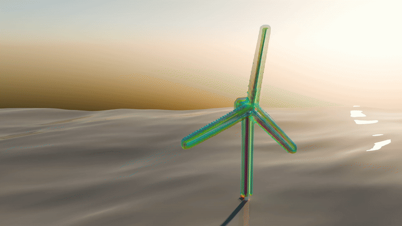
Simulation of a wind turbine based on the immersed boundary method.

On GPU in-situ rendering using PhantomGaze library (no I/O). Flow over a NACA airfoil using KBC Lattice Boltzmann Simulation with ~10 million cells.

DrivAer model in a wind-tunnel using KBC Lattice Boltzmann Simulation with approx. 317 million cells

Airflow into, out of, and within a building (~400 million cells)

The stages of a fluid density field from an initial state to the emergence of the "XLB" pattern through deep learning optimization at timestep 200 (see paper for details)

Lid-driven Cavity flow at Re=100,000 (~25 million cells)

Capabilities

LBM

• BGK collision model (Standard LBM collision model)
• KBC collision model (unconditionally stable for flows with high Reynolds number)
• Smagorinsky LES sub-grid model for turbulence modelling

Machine Learning

• Easy integration with JAX's ecosystem of machine learning libraries
• Differentiable LBM kernels
• Differentiable boundary conditions

Lattice Models

• D2Q9
• D3Q19
• D3Q27 (Must be used for KBC simulation runs)

Compute Capabilities

• Single GPU support for the Warp backend with state-of-the-art performance
• Multi-GPU support using the Neon backend with single-resolution grids
• Grid refinement support on single-GPU using the Neon backend
• Distributed Multi-GPU support using the JAX backend
• Mixed-Precision support (store vs compute)
• Multiple kernel-fusion performance strategies for multi-resolution simulations
• Out-of-core support (coming soon)

Output

• Binary and ASCII VTK output (based on PyVista library)
• HDF5/XDMF output for multi-resolution data (with gzip compression)
• In-situ rendering using PhantomGaze library
• Orbax-based distributed asynchronous checkpointing
• Image Output (including multi-resolution slice images)
• 3D mesh voxelizer using trimesh

Boundary conditions

• Equilibrium BC: In this boundary condition, the fluid populations are assumed to be at equilibrium. Can be used to set prescribed velocity or pressure.

• Full-Way Bounceback BC: In this boundary condition, the velocity of the fluid populations is reflected back to the fluid side of the boundary, resulting in zero fluid velocity at the boundary.

• Half-Way Bounceback BC: Similar to the Full-Way Bounceback BC, in this boundary condition, the velocity of the fluid populations is partially reflected back to the fluid side of the boundary, resulting in a non-zero fluid velocity at the boundary.

• Do Nothing BC: In this boundary condition, the fluid populations are allowed to pass through the boundary without any reflection or modification.

• Zouhe BC: This boundary condition is used to impose a prescribed velocity or pressure profile at the boundary.

• Regularized BC: This boundary condition is used to impose a prescribed velocity or pressure profile at the boundary. This BC is more stable than Zouhe BC, but computationally more expensive.

• Extrapolation Outflow BC: A type of outflow boundary condition that uses extrapolation to avoid strong wave reflections.

• Interpolated Bounceback BC: Interpolated bounce-back boundary condition for representing curved boundaries.

• Hybrid BC: Combines regularized and bounce-back methods with optional wall-distance interpolation for improved accuracy on curved geometries.

Roadmap

Recently Completed

• ✅ Grid Refinement: Multi-resolution LBM with nested cuboid grids and multiple kernel-fusion strategies via the Neon backend.

• ✅ Multi-GPU Acceleration using Neon + Warp: Multi-GPU support through Neon's data structures with Warp-based kernels for single-resolution settings.

Work in Progress (WIP)

Note: Some of the work-in-progress features can be found in the branches of the XLB repository. For contributions to these features, please reach out.

• 💾 Out-of-Core Computations: Enabling simulations that exceed available GPU memory, suitable for CPU+GPU coherent memory models such as NVIDIA's Grace Superchips (coming soon).

• 🗜️ GPU Accelerated Lossless Compression and Decompression: Implementing high-performance lossless compression and decompression techniques for larger-scale simulations and improved performance.

• 🌡️ Fluid-Thermal Simulation Capabilities: Incorporating heat transfer and thermal effects into fluid simulations.

• 🎯 Adjoint-based Shape and Topology Optimization: Implementing gradient-based optimization techniques for design optimization.

• 🧠 Machine Learning Accelerated Simulations: Leveraging machine learning to speed up simulations and improve accuracy.

• 📉 Reduced Order Modeling using Machine Learning: Developing data-driven reduced-order models for efficient and accurate simulations.

Wishlist

Contributions to these features are welcome. Please submit PRs for the Wishlist items.

• 🌊 Free Surface Flows: Simulating flows with free surfaces, such as water waves and droplets.

• 📡 Electromagnetic Wave Propagation: Simulating the propagation of electromagnetic waves.

• 🛩️ Supersonic Flows: Simulating supersonic flows.

• 🌊🧱 Fluid-Solid Interaction: Modeling the interaction between fluids and solid objects.

• 🧩 Multiphase Flow Simulation: Simulating flows with multiple immiscible fluids.

• 🔥 Combustion: Simulating combustion processes and reactive flows.

• 🪨 Particle Flows and Discrete Element Method: Incorporating particle-based methods for granular and particulate flows.

• 🔧 Better Geometry Processing Pipelines: Improving the handling and preprocessing of complex geometries for simulations.